First, a GitHub link for those who prefer reading code. I used fastAI's library, which wraps PyTorch quite nicely for this problem domain.

Given that I'm between internships, I've dedicated this lull in work towards self-learning. Among others, Jeremy Howard's fast.ai deep learning lectures have been an absolute pleasure. One topic of many that captivated me was using deep learning for tabular data through embeddings. While I was aware of gradient boosting for these problems, Jeremy (Howard, not me) suggests that deep architectures can do the job just as well. Before we begin, here are some definitions.

---

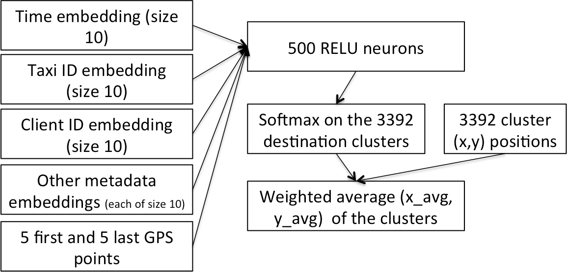
The winning architecture of Kaggle's NYC Taxi Duration Competition

---

An embedding is a way of representing categorical variables numerically. Categorical variables could include non-numeric concepts like season or even low-cardinality numbers such as month. Each category is mapped to an ID, which is associated with a vector. This isn't so different than a one-hot encoding. These vectors are fed through the neural network alongside all the numerical variables. The weights in these vectors are updated as the model learns. The implication is that as the neural net trains, elements with similar traits will have close vectors in Euclidean space.

Tabular data is data that you would expect in CSV format. In particular, we're focusing on time-series data, which involves data points taken chronologically. For these problems, we typically have a goal of predicting the outcome of a future date.

Creating a Tabular Data Model: Predicting Sales

A straightforward example of learning with tabular data is sales prediction from past trends. Luckily, there are tons of Kaggle competitions on this, so I arbitrarily picked Predict Future Sales. It's also a worthy candidate because almost everyone else is using a gradient boosting or similar decision tree approach.

The goal is to predict the sales of each item that a Russian store chain offers for the month after the test data ends. To ensure a worthy comparison between gradient boosting and my approach, I used this kernel as a baseline. It provides a clear benchmark: a root mean square error (RMSE) of 1.0428.

Data engineering isn't the emphasis for this writeup. In short, we transform files like this…

---

item_categories.csv

	item_category_name	item_category_id
0	PC - Гарнитуры/Наушники	0
1	Аксессуары - PS2	1
2	Аксессуары - PS3	2

items.csv

	item_name	item_id	item_category_id
0	! ВО ВЛАСТИ НАВАЖДЕНИЯ (ПЛАСТ.) D	0	40
1	!ABBYY FineReader 12 Professional Edition Full...	1	76
2	***В ЛУЧАХ СЛАВЫ (UNV) D	2	40

shops.csv

	shop_name	shop_id
0	!Якутск Орджоникидзе, 56 фран	0
1	!Якутск ТЦ "Центральный" фран	1
2	Адыгея ТЦ "Мега"	2

sales_train.csv

	date	date_block_num	shop_id	item_id	item_price	item_cnt_day
0	02.01.2013	0	59	22154	999.00	1.0
1	03.01.2013	0	25	2552	899.00	1.0
2	05.01.2013	0	25	2552	899.00	-1.0

test.csv

	ID	shop_id	item_id
0	0	5	5037
1	1	5	5320
2	2	5	5233

---

…Into data that looks like this (many columns omitted for brevity):

	item_id	shop_id	date_block_num	month	year	target	target_lag_1	target_lag_2	target_lag_3	target_lag_12
0	5037	5	34	10	2	0	0.0	1.0	3.0	1.0
1	5320	5	34	10	2	0	0.0	0.0	0.0	0.0
2	5233	5	34	10	2	0	1.0	3.0	1.0	0.0
3	5232	5	34	10	2	0	0.0	0.0	1.0	0.0
4	5268	5	34	10	2	0	0.0	0.0	0.0	0.0

---

The general approach is to introduce lag features. The target was how much was actually sold in the given date_block_num. And the lags correspond to the target 1, 2, 3, and 12 months ago for a given (item_id, shop_id, date_block_num) index. This allows the model to learn how current and past months affect future trends.

Now here's the fun part. Our dataset has a mixture of continuous variables—which feed cleanly into what we expect in a neural net—and categorical variables—which go through the embedding matrices. This data gets fed through 2 hidden linear layers of size 1000 and 500. Finally a sigmoid is applied on the last single-node layer. Architecturally, this is very similar to the winning taxi ride solution above.

To reduce some overfitting problems, I introduced a substantial amount of dropout and L2 regularization. Optimizing based on the root mean square log error (RMSLE) instead of the expected RMSE seemed to stabilize the loss function more easily.

---

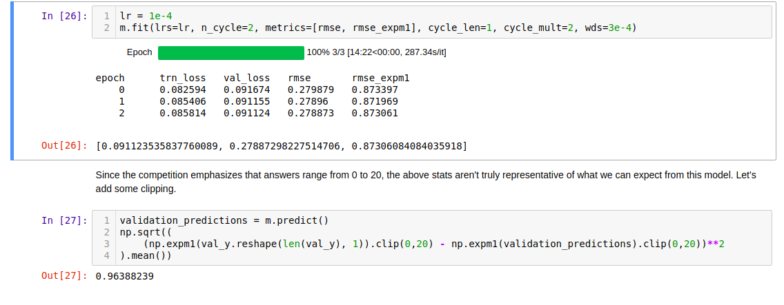
Training the model for 3 epochs

---

I ran this for 3 epochs, and… it worked! The RMSE on the validation set was .9638, and the RMSE on the public leaderboard was .9652, despite some troubles with overfitting. Not only did I outperform the original kernel's score of 1.0428, I placed inside the top 10% of the competition using features that generated only top 25% percent results using gradient boosting. And I didn't spend any time engineering more features.

Should We Always Use Deep Learning?

Although I outperformed the kernel I borrowed, there are a few tree-boosting models that outperformed mine. So what was the cause? One recently available kernel did a lot more feature engineering than I did. Which I suppose is one of the takeaways. While deep learning increased my performance for the limited set of features I used, I spent multiple hours tuning hyperparameters and retraining. XGBoost gave fast feedback and was comparatively easier to configure.

In the end, the training data is just as relevant to success as the model. There were only 212400 rows of data to train on, so adding features would have propelled my model even further and perhaps eradicated the slight overfit.

Is it worth the effort? In production: why not if it really helps? In a Kaggle competition: maybe if the problem is incredibly cool and doesn't have an award of "Kudos."